In this post, I will discuss the different ways in which data can be missing in a (tabular) dataset, and particularly how the Missing at Random (MAR) assumption is ambiguous.

In datasets that have missing values, the missingness mechanism, i.e. the relationship between the data values and which values are missing, often plays a role in determining the optimal data model. In the literature, there are three missingness mechanisms: Missing Completely at Random (MCAR), Missing at Random (MAR), and Missing Not at Random (MNAR). In particularly, I’ve found that the MAR assumption is often defined in subtly different ways, and it’s utility is not always clear. I’ll explain this in detail in this post.

The Typical Missing Value Setup

I’ll start by introducing the most traditional setup in the literature. Let $X = (X_1, \ldots, X_p)$ be random variables representing one complete row of an $n \times p$ dataset of i.i.d. rows. It’s typical then to partition \(X\) into \(X = (X_O, X_M)\) for the observed and missing components of $X$ respectively. By saying that $X$ is complete, I mean that even $X_M$ has true values, just not values that we actually observe. Let $R = (R_1, \ldots, R_p)$ be missing value indicators, i.e.

\[R_i = \begin{cases} 1 & X_i ~~\text{is observed} \\ 0 & X_i ~~\text{is not observed} \end{cases}\]

The so-called missing value mechanism is the distribution $P(R = r \mid X = x)$, i.e. what’s the probability that each \(X_i\) is missing given the (complete) values \(X\). Then, the 3 mechanisms are defined as

• Missing Completely at Random (MCAR): \(P(R = r \mid X = x) = P(R = r)\) i.e. \(R\) is independent of all true values \(X\).
• Missing at Random (MAR): \(P(R = r \mid X = x) = P(R = r \mid X_O) = x_O)\) i.e. \(R\) is independent of \(X_M\) controlling for \(X_O\).
• Missing Not at Random (MNAR): \(P(R = r \mid X = x) = P(R = r \mid X = x)\), i.e. \(R\) is not independent of \(X_O\) or \(X_M\).

MCAR is clearly distinct from the other two types of missingness in that the probability of a given entry being missing is complete random and not related to the value of $X$ at all. The difference between MAR and MNAR, on the other hand, is more subtle. In MAR, the distribution of $R$ is independent of the unobserved entries of $X$, while in MNAR the distribution of $R$ is not independent of any part of $X$, observed and unobserved parts. The distinction between MAR and MNAR was originally made by Donald Rubin, who argued that likelihood-based inference on $X_O$ is equivalent to likelihood-based inference on $X$ only if the MAR assumption holds. For more information on this, see Rubin and Little’s textbook: Statistical Analysis with Missing Data.

Does This Setup Make Sense?

My intuition is that this definition is a little weird. If we would like to partition $X$ into $(X_O, X_M)$, then we actually need to know which indices in $\{1, \ldots, p\} = [p]$ have been observed and which have not. What this means to me is that we actually have random sets $O_R, M_R \subseteq [p]$ defined by

\[O_R = \{i\in[p] \mid R_i = 1\} ~~~M_R = \{i \in [p] \mid R_i = 0\}\]

I’m indexing these sets by $R$ to stress that they depend on the random vector $R$. We can then have realized versions of these sets indexed by a realized binary vector $r$. This does not affect the definitions of MCAR and MNAR, but it does affect the definition of MAR. MAR now becomes

\[\textbf{MAR:} ~~P(R = r \mid X_{O_r} = x_{O_r}, X_{M_r} = x_{M_r}) = P(R = r \mid X_{O_r} = x_{O_r})\]

In words, this means that the probability of a given observed/missing pattern $r$ depends only on the features that are observed (according to $r$). Here’s one way to think about it. We are asking for the conditional probability that $R$ equals $r$, but the sets $O_r$ and $M_r$ change depending on the choice or $r$, so which features are conditionally independent of $R$ change for each choice of $r$. For example, if $r_1 = 0$ and $r_i = 1$ for all other $i$, then the probability that feature 1 is missing and all others are observed is independent of the true value $x_1$ conditioned on $x_2, \ldots, x_p$. However, now change to $r_1 = 1$ and the probability that feature 1 is observed (and all others are also observed) now is not independent of $x_1$!

My takeaway from the above is that this definition of MAR is a bit strange and definitely hard to wrap your head around. This is the definition that Rubin showed is useful, though (since in theory we only need to maximize the likelihood of the observed data to train a model), so making an effort to use this definition is enticing. However, there are two problems with using this definition, other than that it’s confusing. First, it is not clear how to practically maximize the likelihood using only the observed entries, since the number of features can change for each row. Second, it is actually impossible to test if data is MAR or MNAR using this definition, since the distinction depends only on the values we don’t observe. It seems to me then that this definition is useful in theory, but maybe not so useful in practice.

Other Definitions of MAR

Interestingly, when people explain MCAR/MAR/MNAR through examples instead of mathematically, the definition of MAR seems to change. In MAR, instead of the missing probability depending on only the observed data, it is often worded that the missing probability of a given feature only depends on other observed variables. This way of thinking is often supported by examples, like the one in this book: a weighing scale that is more or less likely to fail based on the surface which it has been placed on. Thus, if we condition on the observed surface type, the missingness does not depend on the actual weight of the object. We can’t condition on the actual weight at all without the missingness becoming MNAR.

Mathematicaly, let $i \in [p]$, and let the sets $O, M$ be realized sets of observed and missing indices respectively that partition $[p] \setminus \{ i \} $ (notice we’re excluding $i$), then we have

\[\textbf{MAR}: P(R_i = r_i \mid X_O = x_O, X_M = x_M) = P(R_i = r_i \mid X_O = x_O)\]

Of course, the dataset is MAR if each feature is MAR. Notice that this is a slightly stronger assumption than the previous MAR definition, since now the probability that $R_i = r_i$ must be independent of all other observed components AND $X_i$, regardless of whether $r_i$ equals 0 or 1. This means that Rubin’s theorem for maximizing the observed likelihood still holds, yet we still don’t have a test for this assumption, so it is still not particularly useful in practice. I would argue that it is more useful than the previous definition, though, because it is often times easier to argue that the assumption holds just from prior knowledge of the data gathering process since the definition follows much more easily from common examples.

An even stronger MAR assumption is to assume that the partition of missing and observed features does not change row-by-row. In this setup, the partition actually becomes always observed variables and partially observed variables, and the MAR assumption is that a given missing indicator is independent of the partially observed variables given the always observed variables. This assumption is definition significantly stronger than the previous MAR assumptions, but that comes with the benefit of being able to test it. One way to do such a test would be to build a logistic regression model predicting $R_i$ from the always observed variables, and then compare this to the logistic regression model predicting $R_i$ from all observed variables in each row.

In the recent literature, it has actually become popular to define MAR in this last way not using probability statements but on causal graphs. Two examples are the following papers from NeurIPS 2021: MIRACLE and GINA. The idea is that the missingness random variables $R_i$ are somehow caused by other variables in the dataset, and these relationships can be represented in a graphical structure with nodes for each $X_i$ and $R_i$. Below is one example of such missingness graphs from the MIRACLE paper.

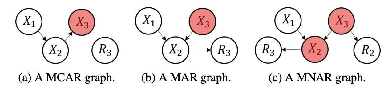
The white nodes are always observed, and the red nodes are partially observed. What I don’t like about the causal graph approach is that it forces causal relationships into the $X_i$ and $R_i$ space. The possibility of having confounding features not in the dataset but that actually cause missingness makes enforcing causal relationships delicate, more so than simply analyzing correlation structures. Nonetheless, it seems to be popular for modelling MNAR data, and successful based on the strong results from the MIRACLE paper.