In this post, I’m going to introduce the concept of a neural network at a level appropriate for someone with the mathematical background typical of a Statistics student. I’ll start by reviewing linear regression and then showing how a multi-layer perceptron (MLP) is a natural extension.

If you have visited the home page of my website, you’ve seen that I’m a Statistics PhD student, and that I’m interested in deep learning. Since I’ve started my PhD, I’ve noticed that many Statistics students do not have a good understanding of neural networks, often thinking of them as mysterious black boxes. I think part of the reason for this perception is that neural networks are often explained too abstractly, omitting how the neural network actually works, or too intricately, in a way that only makes sense to someone involved in the deep learning literature. The goal of this post, then, is to explain neural networks at an introductory level but from the perspective of a Statistics student, hopefully providing a good introduction at an appropriate level for someone with some math background.

Below are two pictures that you would see that describe neural networks.

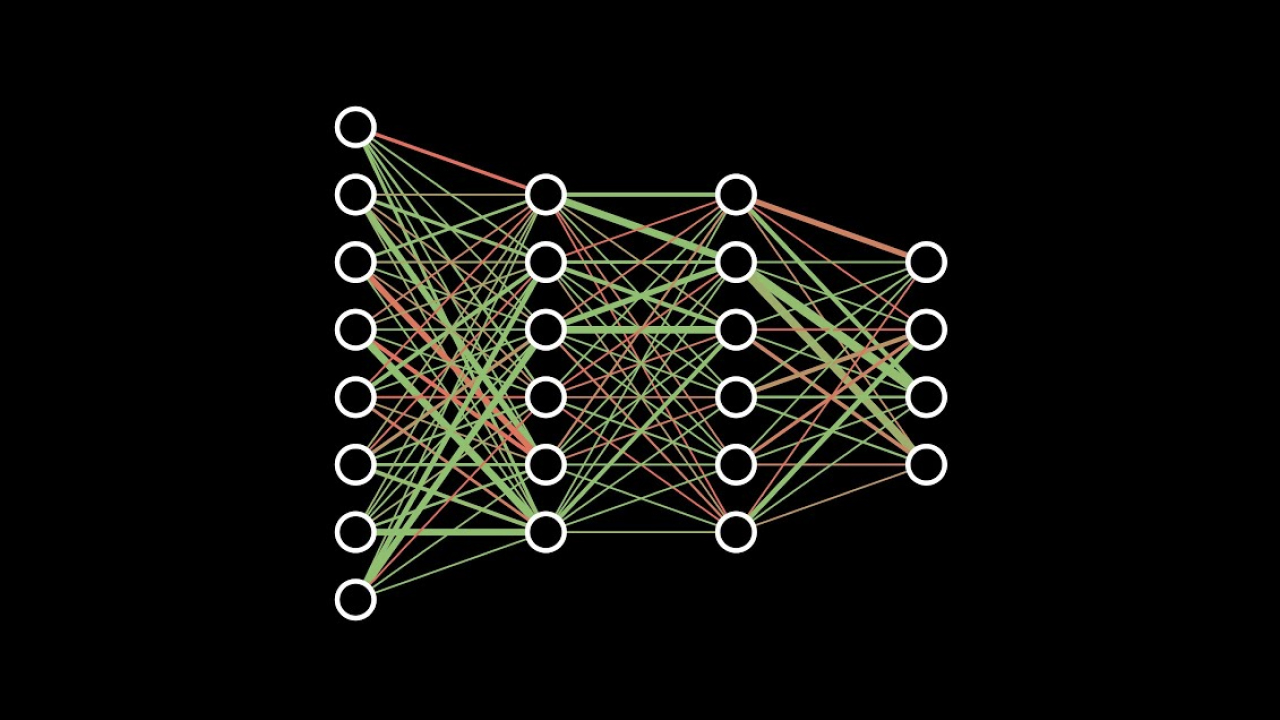
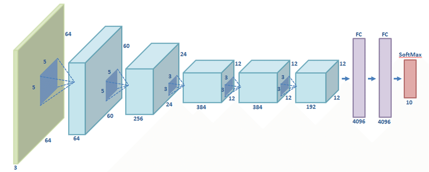
On the left is a picture of a neural network shown in the 3 blue 1 brown neural networks video, a very popular introduction video to neural networks. While the video is a good high level introduction to neural networks, it presents neural networks from a biological perspective, comparing to neurons in the brain. While this can serve as a useful metaphor, I think it can sometimes make neural networks seem more complicated then they actually are. Meanwhile, the picture on the right is an overview of the AlexNet, one of the most famous neural network architectures. In this case, I think it is very hard to understand how such a neural network works without having a baseline understanding of the deep learning literature.

Rather than learning about neural networks from high level tutorials or research papers, I think the best way to first introduce neural networks for someone with math background is to start with linear regression. Suppose we have a dataset of \(n\) data samples and \(p\) features represented as a matrix \(X \in \mathbb{R}^{n \times p}\) and labels \(y \in \mathbb{R}^n\). In a linear regression model, we would model the data as \(Y = X w + \epsilon\) where \(w \in \mathbb{R}^p\) is a vector of feature coefficients and \(\epsilon \in \mathbb{R}\) is a vector of residuals. We can find the optimal \(w\) by minimizing the sum of squares residuals:

$ \hat{w} = \mathrm{argmin}_w || y - Xw ||_2 $

Taking the gradient with respect to \(w\) we can find the minimizer to be the ordinary least squares solution \(\hat{w} = (X^T X)^{-1} X^T y\). I kinda rushed through this because if you’ve studied Statistics, this is surely very familiar.

Let’s now consider doing something slightly different. Suppose that \(W_1 \in \mathbb{R}^{p \times d}\) and \(W_2 \in \mathbb{R}^d\), then we could model our data as \(Y = (X W_1) W_2 + \epsilon\). This doesn’t add anything, though, because we could simply let \(w = W_1 W_2\) and we would have the same linear regression model as before. To make this model interesting, let’s introduce a simple nonlinear function, which in the deep learning community is called a Rectified Linear Unit, or ReLU. The function is defined as

$ \text{ReLU}(x) = \begin{cases} x & x > 0 \\ 0 & x \leq 0 \end{cases} $

Now let’s model our data as \(Y = \text{ReLU}(X W_1) W_2 + \epsilon\). This is a simple neural network! It’s usually called a Multi-Layer Perceptron, or MLP. This subtle addition to the network turns out to be very important and what distinguishes a simple neural network from linear regression. The main reason for this is that the ReLU function is nonlinear, making the neural neural model a nonlinear model distinct from the previous linear model. While this nonlinear model is certainly more complex and less interpretable than a linear model, it has the benefit of being able to model nonlinear relationships in the data, making it a more expressive model. In fact, such a neural network has the ability to approximate any continuous function, as shown by the universal approximation theorem. Further discussion of the universal approximation theorem is beyond what I’d like to discuss here, so the main takeaway is this simple MLP neural network is actually pretty powerful.

There are still a few questions that we need to address about our simple MLP network. First, how do we actually fit the model? With the linear regression model there is a nice closed-form solution by taking a gradient of the sum of squared residuals. In the MLP model the sum of squares residuals is

$||y - \text{ReLU}(X W_1) W_2||_2$

We need to minimize this with respect to \(W_1\) and \(W_2\), and there’s no closed form way to do this. Thus, we need to turn to iterative solutions in order to fit the model. For neural networks, we typically turn to gradient descent. We first specify a loss function, which I’ll now use the mean squared error (MSE) instead of the sum squared error:

$L(y, X) = \frac{1}{n}||y - \text{ReLU}(X W_1) W_2||_2$

Gradient descent then iteratively finds new parameters \(W_1^t\) and \(W_2^t\) from the previous iterations parameters \(W_1^{t-1}\) and \(W_2^{t-1}\) as

\[\begin{align*} W_1^t &= W_1^{t-1} - \eta \frac{\partial L}{\partial W_1} \\ W_2^t &= W_2^{t-1} - \eta \frac{\partial L}{\partial W_2} \end{align*}\]

where \(\eta\) is a small, constant learning rate. While gradient descent isn’t guaranteed to produce optimum parameters, it turns out to be pretty good in practice with neural networks. This leads to a second question about this neural network model: if the goal is to produce a nonlinear model that is more expressive, why choose a neural network instead of other nonlinear models? One reason neural networks are great is that you can add any functions to them as long as those functions are differentiable. This is because gradient descent can update the parameters of the model as long as the loss function is differentiable with respect to each parameter.

Perhaps at this point it’s worth doing an example more abstract than the simple MLP. Let’s say we have the following model still for data matrix \(X\) and labels \(y\):

\[\begin{align*} h_1 &= f_1(X, w_1) \\ h_2 &= f_2(h_1, w_2) \\ h_3 &= f_3(h_2, w_3) \\ \hat{y} &= f_4(h_3, w_4) \end{align*}\]

In this abstract model, \(w_1, w_2, w_3,\) and \(w_4\) are parameters that should be learned by the model, and \(f_1, f_2,\) and \(f_3\) are some functions that are differentiable with respect to both their inputs as well as their associated parameters. Then given a loss function \(L(y, \hat{y})\) we can find the necessary derivatives for gradient descent via the chain rule:

\[\begin{align*} \frac{\partial L}{\partial w_4} &= \frac{\partial L}{\partial \hat{y}} \frac{\partial \hat{y}}{\partial w_4} \\ \frac{\partial L}{\partial w_3} &= \frac{\partial L}{\partial \hat{y}} \frac{\partial \hat{y}}{\partial h_3} \frac{\partial h_3}{\partial w_3} \\ \frac{\partial L}{\partial w_2} &= \frac{\partial L}{\partial \hat{y}} \frac{\partial \hat{y}}{\partial h_3} \frac{\partial h_3}{\partial h_2} \frac{\partial h_2}{\partial w_2} \\ \frac{\partial L}{\partial w_1} &= \frac{\partial L}{\partial \hat{y}} \frac{\partial \hat{y}}{\partial h_3} \frac{\partial h_3}{\partial h_2} \frac{\partial h_2}{\partial h_1} \frac{\partial h_1}{\partial w_1} \end{align*}\]

Okay, let’s recap. We showed that we can take a linear regression model and modify it slightly to make a simple MLP model. The motivation for doing this was to create an extension of linear regression that is nonlinear so that it can model a more diverse set of data/tasks. We’ve seen that this model can be fit using gradient descent, and similarly that gradient descent can be used to fit any model that is built using differentiable functions. This makes neural networks an extremely flexible set of models that can be used to model almost any kind of data and/or task.